Mechanisms and limits of exponential growth
Authors and date
- Submitted on: May 31th 2021
- Martine Olivi; Research Fellow at Inria
Always faster
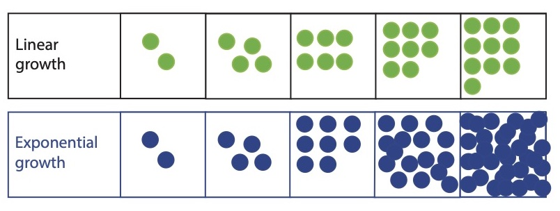
This is how exponential growth can be described. Linear growth and exponential growth are two simple and relevant mathematical models, essential reference points in the jungle of evolutionary behavior observed in the real world. In linear growth, the increase per unit of time is a fixed number: for example, the diameter of a tree grows by 5 cm per year, regardless of its size. In an exponential growth, the increase per unit of time is proportional to the quantity: for example the evolution of the number of people infected by a virus depends on the number of infected people. This is the snowball effect.
See the mathematical formulation
If \(x_n\) denotes the quantity measured in year \(n\), and \(a\) the proportionality coefficient or growth rate, the exponential growth is expressed by the relation
\(x_{n+1}-x_n= a\, x_{n}\)
The sequence \((x_n)\) is a geometric sequence: \(x_{n+1}= (1+a)\, x_{n}\) of ratio \(1+a\) greater than \(1\), the famous \(R\) of epidemiology models. When \(a\) is positive, the larger the quantity, the more it increases.
> « Faster, bigger, better: for several decades, Moore's laws have governed the exponential growth of computer science performance, with a stronger sense of progress than in any other sector. » Cédric Villani.
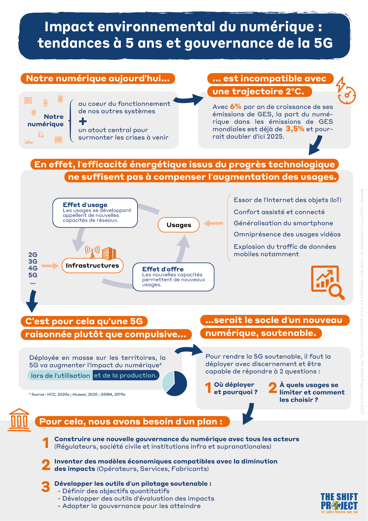
The share of global GHG emissions due to digital technology is currently growing at 6% per year, i.e. it is multiplied by 1.06 each year. After two years, it will be multiplied by \(1.06^2=1.1236\). For example, the amount of data exchanged on mobile networks doubles every 3 years! Now we can see a bit more clearly, we know that a quantity that doubles at regular intervals will quickly become huge, as illustrated by the Sissa chessboard problem, or the water lily growth problem1. Calculating the doubling time of a quantity allows to better imagine an exponential growth. At a rate of 6% per year, the share of global GHG emissions due to digital technology should therefore double within 12 years (\(1.06^{12} = 2.0122\)). This would mean that in the next 12 years, digital technology would emit as much GHG as it has emitted to date since the beginning of the digital revolution. Its emissions would then represent 7% of the world's GHG emissions, whereas they are currently at 3.5%. And that's without taking into account the probable increase of this growth rate 2.
But why does this dizzying growth continue when technical progress is making our equipment more and more energy efficient? This can be explained in the following way 2: the improvement of technical performances leads to an increase in uses, which in turn leads to new improvements, etc. It is a loop. This is a positive feedback loop that stimulates growth. The increase in energy consumption caused by the increase in use largely offsets the energy savings due to technical improvements. This is called a rebound effect (see concept sheet "The rebound effect"concept sheet "The rebound effect" ).
Vicious or virtuous circle?
According to Olivier Hamant, Director of Research at INRAE,
> Feedback is a key concept for understanding life, from the cell to the planet.
This concept is also more relevant than that of causality to describe the behavior of a complex system. We distinguish between positive feedbacks which cause an accentuation of the phenomenon, or even a runaway. A small disturbance can then trigger an exponential growth of the quantities involved. Negative feedbacks, on the other hand, are opposed to the phenomenon that generated them and can regulate it, or reduce it to nothing. *system]: a set of elements interacting with each other according to certain principles or rules (wikipedia)
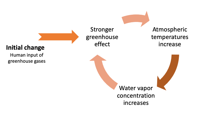
In climate models, there are many feedback loops. A classic example is that of water vapor. The increase of CO2 in the atmosphere (initial perturbation) leads to an increase of the global temperature. As the temperature increases, the concentration of water vapor in the atmosphere increases in turn. There is more moisture in the air. But water vapor is a powerful greenhouse gas. If the amount of water vapor in the atmosphere increases, it will cause the temperature to rise and so on.
The case of clouds is particularly interesting because it is a challenge for climate scientists. Clouds in the lower atmosphere reflect part of the solar radiation and contribute to the cooling of the planet, while clouds in the upper atmosphere contribute to the greenhouse effect. But the changes in the cloud layer due to global warming are still poorly understood, and scientists do not know to date whether clouds ultimately contribute to a positive or negative feedback3.
A video from SimClimat4 shows the importance of taking these feedback phenomena into account in climate models and explains how to check that these models have been correctly calibrated, i.e. that the parameters outside the model have been correctly chosen.
Flatten the exponential.
> "I can tell you as a biologist that all the exponential curves that we observe in the plant world and in the animal world among living beings, always end up extremely bad. The case where it goes less badly is when there is a stabilization."
This was said by Jean Dorst, a French ornithologist, in the program Demain la terre of 13/04/19745. But how to stabilize growth? How to flatten the exponential?
The Belgian mathematician Pierre-François Verhulst (1804-1849), looked for a mathematical answer to this problem, raised by Malthus at the end of the 18th century, who was worried about the exponential growth of the human population. Verhulst proposed another form of growth, the logistic growth. What this model tells us is that exponential growth confronted with limits (food, space) regulates itself.
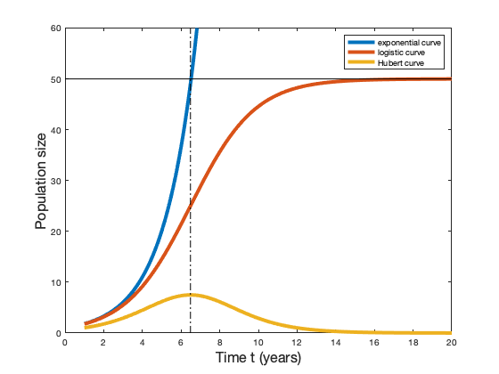
Verhulst's model is in continuous time: time is represented by a real variable, \(t\), and the population at time \(t\) is given by a mathematical function, i.e. a process which corresponds to the variable \(t\) and a quantity noted \(f(t)\). The representative curve of the function \(f\) has a characteristic \(S\)-shape, also called sigmoid. It starts to grow like an exponential when the population is still small, then the curvature reverses and the curve approaches a limit value \(K\) without ever reaching it.
See the mathematical formulation
The function \(f\) is the solution of an equation that relates the instantaneous rate of change of the population to the population itself. The instantaneous rate of change must be thought of as the speed of growth of the population and it corresponds to a mathematical operation, the derivative or differential, noted \(f'\). The logistic equation is:
\(f'(t)= a\, f(t)\, (1- f(t)/K).\)
The exponential growth is regulated by a negative feedback (the sign - in the equation), which involves a parameter \(K\), called the carrying capacity. When this capacity tends to infinity, the negative term tends to \(0\) and we find the exponential growth:
\(f'(t)= a \,f(t).\)
In practice, the two parameters \(a\) and \(K\) must be adjusted from real data in the same way as one adjusts the slope of a line passing through points that appear to be aligned (linear regression). The instantaneous rate of change, the derivative function \(f'\), has a bell-shaped representative curve, symmetric about its maximum, known as Hubert's curve.
The American geophysicist Marion King Hubert found the logistic function relevant to represent the cumulative extraction of oil, which is clearly limited by the total amount of existing oil. Hubert deduced that oil production, represented by the bell-shaped curve that now bears his name, goes through a peak before falling. He even estimated that oil production in the US would peak in 1970!
The logistic model, the flagship model of population dynamics, has also been used to analyze the depletion of resources or to illustrate the diffusion of an innovation. But of course such a simple model only gives a rough representation of reality, and does not allow precise predictions. However, it allows to estimate time scales and raises fundamental questions 6.
Models on a global scale
> Essentially all models are wrong but some are useful. George E. P. Box
One of these fundamental questions is the following: planetary resources being limited, will the human population nicely follow a logistic curve and stabilize around its maximum carrying capacity or exceed it and then fall more or less abruptly?
To answer this question, researchers at MIT designed the mathematical model World3, which was used to write the book "The Limits to Growth" (1972). This model comes from a very young discipline, systems dynamics, born in the 1950s at MIT. The advent of the first computers allowed researchers to tackle complex problems, here on a global scale and over long periods of time. According to this model, the exponential growth of industrial production could indeed lead to an overshoot of the carrying capacity, and a collapse, which should be understood as a more or less rapid fall in population and production.
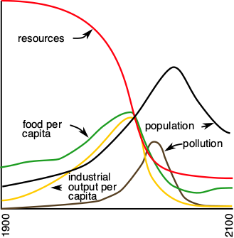
In World3, the "world system" is represented by reservoirs (population, capital, natural and non-natural resources, wealth, pollution), which communicate with each other through material flows and positive or negative effects. This model is based on the hypothesis of a maximum capacity of the planet to produce certain resources that are indispensable to humanity. The interactions are governed by simple mathematical laws, such as logistic growth.
It is therefore an extremely simplified model, which brings together very different realities under the same banner. There is also no rigorous way to verify the calibration of the model: the choice of key parameters and the different feedbacks. However, it fits quite well with the real measurements observed since, and it provides interesting clues like the inertia of the world system or the major role of pollution in a number of negative feedbacks. As underlined in this video from Heu?reka7, it carries a message that speaks to scientists: humanity must set development goals in accordance with the constraints of nature. It also promoted a systemic approach to environmental issues.
From the 1950s onwards, the systems approach, until then reserved for engineering, spread to other fields: the evolution of human development, as we have just seen, but also the study of climate, which should not be confused with weather. In the study of climate, we are interested in averages and statistics, not in localized or specific events. Historically, the first atmospheric model dates from 1950, and was tested on the first existing computer, the ENIAC. Since then, climate models have continued to grow and now include five main components: the atmosphere, the continental surfaces, the hydrosphere, the cryosphere, and the biosphere. These components exchange water, heat, chemical compounds, ...
Contrary to the World3 model, the equations governing the interactions between the different characteristic quantities are the equations of physics, and the key parameters are calibrated on historical data. The numerical resolution of these complex equations requires the division of the surface of the earth, the oceans and the atmosphere into small cubes called meshes. The smaller the grid cells, the more accurate and reliable the calculations. The number of grid cells used in climate models has increased exponentially over the years! Today, about forty different models are developed in the world, including that of the Institut Pierre-Simon Laplace (IPSL) in France. The IPSL proposes a simplified version of its model for educational use8.
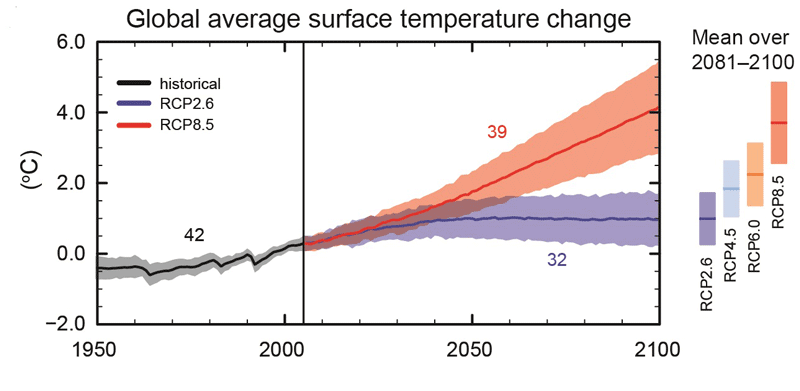
GHG emissions appear as perturbations outside the system, and these models simulate the different scenarios of reduction of these emissions, which have been presented in the different IPCC reports. These models are imperfect, because some physical phenomena are still poorly understood and because of the uncertainties linked to numerical modelling. But here again, the objective is not to make quantitative forecasts, but to obtain orders of magnitude, which allow us to understand the influence of our development choices on the climate. And they play this role perfectly.
Lexicon
Instantaneous increase: variation of a quantity which varies in the course of time related to an infinitesimal variation of time
Biosphere: all living organisms in the air, on land and in the oceans
CMIP: Coupled Model Intercomparison Project. This project aims to carry out climate simulations in a coordinated way between different research groups allowing a better estimation and understanding of the differences between climate models wikipedia
Cryosphere: land or sea ice, snow cover
Hydrosphere: oceans, lakes, rivers, groundwater ...
Feedback: a feedback is the action in return of an effect on the mechanism that gave it birth.
System: a set of elements that interact with each other according to certain principles or rules. A system composed of a large number of elements and interactions is called complex.
Bibiography
Articles
- Cedric Villani. L’informatique durable n’existe pas encore [online]. Libération, 2021. Available at the Libération website [20/07/2021]
- Martine Olivi. Des expériences pour mieux appréhender la croissance exponentielle [online]. Pixees, 2020. Available at Pixees [20/07/2021]
- Olivier Hamant. La rétroaction, un concept clé pour comprendre le vivant, de la cellule à la planète [online]. Inrae, 2020. Available at the Inrae website [20/07/2021]
- Laurent Li. Les rétroactions sont-elles prises en compte dans les modèles? [online]. Le climat en questions (IPSL), 2014. Available at Le climat en questions site [20/07/2021]
- Sylvain Barré. Inverser la courbe [en ligne]. Image des Maths (CNRS), 2014. Available at Images des Mathématiques [20/07/2021]
- José Halloy. L’épuisement des ressources minérales et la notion de matériaux critiques [en ligne]. La rue nouvelle, 2018. Available at revuenouvelle.be [20/07/2021]
- Daniel Perrin. La suite logistique et le chaos [en ligne]. Département de Mathématiques d'Orsay, 2008. downloadable from [20/07/2021]
Infographic
- Shift Project. Digital environment impact, 5-year trend and 5G governance, 2021, url
Books
- Donella Meadows, Jorgens Randers, Dennis Meadows. Limits to Growth - The 30-Year Update [online]. Dennis Meadows, 2004. Available at [20/07/2021]
Web pages
- Insightmaker, The World3 Model Classic World Simulation, url
- Laboratoire de Météorologie Dynamique, SimClimat: un logiciel pédagogique de simulation du climat, 2020 update, url
Podcasts
- Hélène Combris. Le jour du dépassement recule de trois semaines. France Culture, Covid-19, retour sur Demain la terre of 13/04/1974, updated 2020 url [20/07/2021]
Reports
- GreenIT, Empreinte mondiale du numérique, 2019 url
- Shift project, Déployer la sobriété numérique, 2020, url
Videos
- Rodolphe Meyer, Le réveilleur. Modèles climatiques, 2016, 10:30. url
- Institut Pierre-Simon Laplace (IPSL), Tutoriel SimClimat no 3: Les rétroactions climatiques, 2020. 9:16. url
- Gilles Mitteau, Heu?reka: Modéliser l'avenir de l'humanité, 2020. 1:13:15. url
Sources
-
Martine Olivi, Des expériences pour mieux appréhender la croissance exponentielle, Pixees, 2020, url ↩
-
Shift project, Impact environnemental du numérique:tendances à 5 ans et gouvernance de la 5G, 2021, url ↩↩
-
Laurent Li, Les rétroactions sont-elles prises en compte dans les modèles ?, Le climat en questions (IPSL), 2014, url ↩
-
Institut Pierre-Simon Laplace (IPSL), Tutoriel SimClimat no 3: Les rétroactions climatiques, 2020, url ↩
-
France Culture, Covid-19 : le jour du dépassement recule de trois semaines par Hélène Combris (return on Demain la terre of 13/04/1974), updated 2020 url ↩
-
José Halloy, L’épuisement des ressources minérales et la notion de matériaux critiques, La rue nouvelle, 2018, url ↩
-
Gilles Mitteau, Heu?reka: Modéliser l'avenir de l'humanité, 2020 url ↩
-
Dynamic Meteorology Laboratory, SimClimat: un logiciel pédagogique de simulation du climat, 2020 update, url ↩