Numerical simulation, a central tool for the environment
Authors and date
- Submitted on: September 5th 2021
- Eric Blayo; professor of applied mathematics, Grenoble Alpes University
Introduction
When talking about numerical simulation for the environment, one first often thinks of the climate projections that the IPCC regularly presents, as already mentioned in this MOOC. But there are in fact many environmental issues for which numerical models provide a crucial aid to understanding and decision-making.
This concept sheet will attempt to clarify what numerical simulation is, beyond the more or less indefinite idea that we may all have, and how it has developed in the environmental field for many applications.
Modelling: a mathematical vision of the real world
Modelling a system, whether it is the structure of a bridge, the flow of customers at the checkout of a supermarket, or the earth's climate, means above all formalising the main principles governing its behaviour and translating them into mathematical equations. In the so-called "hard" sciences, these principles are fairly well known: conservation of mass and/or energy, chemical transformations, relations between species, etc. In fluid mechanics, which is at the forefront of many environmental issues (atmosphere, ocean, rivers, etc.), the work of great scientists such as Euler, Fourier, Navier, Stokes, Coriolis and Boussinesq has laid the foundations of such equations for two centuries. For other types of complex systems such as vegetation or the economy, this mathematical description is less advanced, even if knowledge is constantly progressing.
However, the complexity of these mathematical models is often such that it is impossible to solve their equations exactly1. However, one can look for approximate solutions (but not approximate!) thanks to the techniques of numerical simulation. The basic idea is to divide the object of interest (a bridge, a mechanical part, the earth's atmosphere) into "elementary bricks" (the mesh of the object) and to look for a value of the physical quantities of interest in each mesh, replacing the equations by a simplified version (the discretized equations) involving only the values in the neighbouring meshes, linked by arithmetic operations2. In this way, each complex initial equation is replaced by a system of very simple equations (one per mesh), whose unknowns are the values of the physical variables (temperature, chemical concentrations, etc.) in each mesh. All that remains is to solve this set of simple equations, which may require a powerful computer if a large number of grid cells are to be used3.
This methodology is always more or less the same, whether you are interested in simulating the Earth's climate or a biscuit dough flow in a food factory.
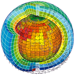
Figure 1 Three-dimensional mesh of the atmospheric component of a climate model. The colours represent temperature and the arrows represent wind. Vincent Landrin, after Laurent Fairhead/LMD/CNRS.
The digital model: video game or scientific tool?
At this stage, we have a digital tool to provide an avatar of a real system. However, there is no guarantee of its quality: clicking on the "start" button will always cause it to create results, which can be enhanced by beautiful 3D animations. But the quality of a visual rendering does not determine the scientific quality (even if the rendering can of course be important to help the scientist understand and exploit the results of the simulation, as well as for mediation purposes towards the general public). Several steps are therefore still necessary for the digital model to become a real scientific tool.
A first major challenge is to ensure that the numerical solution obtained is a good approximation of the solution of the original complex equations. This assurance is achieved by various mathematical techniques used throughout the modelling and calculation process.
For the numerical model to be realistic, it is also necessary to "tune its knobs", i.e. the physical and numerical parameters involved in the model whose values are not necessarily well known. This adjustment is carried out by comparing the results of the model with real-life observations and/or different physical criteria. Very sophisticated mathematical techniques (inverse methods or data assimilation) can be used to determine such optimal settings. This is what all weather forecasting centres do on a daily basis, for example, by "assimilating" millions of atmospheric measurements taken over the last 24 or 48 hours, in order to determine the current state of the atmosphere, which will be the starting point for the forecast for the following days.
Finally, a particularly useful piece of information for the user of a numerical model is the level of confidence he can have in its results. A good model therefore also seeks to provide an estimate of the uncertainty in its results, which can range from a simple qualitative indicator (a confidence index) to a probabilistic description of the range of possibilities.
Numerical simulation for climate
Because of its obvious practical interest, weather forecasting was a precursor field of numerical simulation. Since the first numerical weather prediction by Charney and Von Neumann4 at the end of the 1940s, which was inspired by the visionary work of Richardson5, models were constantly improved, and this know-how spread among geophysicists and greatly accelerated the development of numerical models in related disciplines: the first models of ocean circulation and climate in the 1970s, then hydrology, glaciology, etc.
Describing the climate means explaining the functioning of its main components: atmosphere and ocean, but also cryosphere, rivers, soils, biosphere, etc. So many "compartments" whose interactions must also be explained (exchanges of energy, water, carbon, etc.). Let's insist on a fundamental point: even if it is intrinsically impossible to predict the weather beyond a timeframe of the order of 15 days6, its statistical behaviour (i.e. the climate) is, on the other hand, completely predictable several decades in advance. This is of the same order as accurately predicting the evolution of the average temperature in a pan of water on a gas cooker according to the flame setting, while we are unable to anticipate the exact behaviour of each molecule.
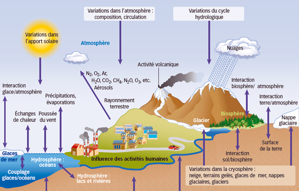
Figure 2 The main components of the climate system and their interactions. Vincent Landrin (source: 4th IPCC report)
The computer implementation of climate models is a real challenge. The behaviour of the climate system, even on a large scale, is largely influenced by smaller-scale phenomena. It is therefore theoretically necessary to use a sufficiently fine spatial resolution, ideally of the order of a few kilometres for the atmosphere, and even finer for the ocean. But the number of discretised equations to be solved would then far exceed the capacities of the most powerful supercomputers. The resolution of climate models is therefore determined for the time being, and will continue to be for a long time, by the computing power available. It is currently relatively low: of the order of 50 to 100 km horizontally for the atmosphere and the ocean, and a few tens to hundreds of metres vertically. The finest spatial scales are not present in these models, and their effect on the larger-scale climate can only be simulated imperfectly, using ad hoc terms added to the equations. But even with this insufficient resolution, the models calculate the evolution of several tens to hundreds of millions of variables, over periods of tens of years, at intervals of a few minutes or tens of minutes, which represents a gigantic volume of calculation.
Numerical climate models are tuned and validated by comparing their results with the available observations, particularly the many from recent decades. Once they have been fine-tuned, they can then provide projections of possible climate developments in the decades, or even centuries, ahead. These studies are coordinated at international level by the IPCC, created in 1988 by the UN. This Intergovernmental Panel on Climate Change provides summary reports on scientific knowledge about climate change. Several "possible futures" of human societies (economic and demographic development, energy choices, changes in individual behaviour) are translated into greenhouse gas emission scenarios. Research centres around the world then simulate the resulting climate changes with their various models. A global synthesis is then produced in order to identify reliable trends and to quantify the uncertainties surrounding these trends.
Numerical simulation and environment
Numerical models have countless applications in environmental fields, whether for short-term forecasting (meteorology, air quality, flood risk, etc.), medium- or long-term forecasting (seasonal forecasting of the monsoon or El Niño, climate projections, etc.), or impact studies (how will silting up evolve if a dyke is built? What areas are at risk if a dam breaks?)
Beyond water and air, numerical models are also omnipresent in the field of living organisms: ecological models studying the evolution of populations of different species, marine biogeochemistry, vegetation, agriculture (optimisation of inputs, harvest forecasting, etc.). They are also important tools for understanding and decision-making for public policies concerning, for example, the organisation of land and transport.
Even if there are still scientific barriers to modelling and simulation, digital technology therefore plays a central role in analysing many environmental issues (first and foremost climate change), and in helping to raise public awareness and develop political action.
-
These are often partial differential equations, for which exact solutions are only known in particularly simple cases. ↩
-
One method is to replace the derivatives by growth rates. Thus the derivative along the direction x of the temperature at the centre of a mesh number i can be approximated by the rate of increase of the temperatures of the left (i-1) and right (i+1) meshes: (dT/dx)i ~ (Ti+1-Ti-1)/(xi+1-xi-1) ↩
-
An operational weather model commonly has several tens or hundreds of millions gridcells. ↩
-
Charney J., R. Fjörtoft and J. Von Neumann, 1950: Numerical Integration of the Barotropic Vorticity Equation. Tellus A. 2. 10.3402/tellusa.v2i4.8607. ↩
-
Lewis Fry Richardson, 1922: Weather Prediction by Numerical Process, Cambridge University Press. ↩
-
This is the "butterfly effect" made famous by Edward Lorenz (1917 - 2008), which illustrates the chaotic character of the dynamics of the atmosphere. The same is true for the ocean on slightly longer time scales. ↩